
Authors: Hoang Long Dang and David Rawlinson
UPDATE: Full HRM-Agent paper now available.
When the Hierarchical Reasoning Model was released, we were very excited about its combination of small size and impressive reasoning abilities. These qualities seem to be enhanced by recurrent processing, but with a surprisingly simple gradient update based on the converged recurrent forward state — turning a weakness of recurrent networks into a feature. We wrote a previous post about it, and judging by the reception it seems many of you were excited about it too (if you haven’t seen it yet, check out Alexia Jolicoeur-Martineau’s Tiny-Recurrent Model which was released just this week).
Since then we have been working to adapt HRM to a Reinforcement-Learning (RL) context. Our motivation for this is primarily to create an RL Agent which has open-ended reasoning and planning abilities, and then demonstrate it in a series of increasingly complex tasks.
I’m pleased to report we have now succeeded in creating a HRM-Agent and capturing evidence of long-term reasoning (planning) when trained only using rewards (RL) — preliminary results below.
This post will describe what we’ve done and we’ll follow up with a preprint paper as soon as all experiments are complete. [EDIT: preprint is now available].
From fully-observable, static problems to partially-observable, dynamic environments
All the problems demonstrated in the HRM paper are static and fully observable. This means that the HRM model reasons about the entire problem, and produces the entire solution in one stream of output. It isn’t possible for the problem to change while it is being solved, or for new information to be integrated into the reasoning process.
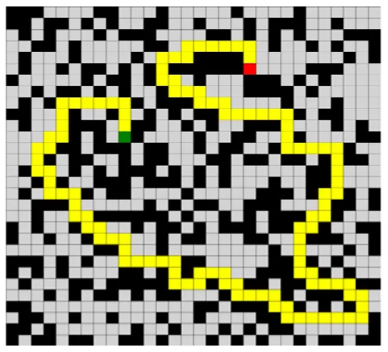
For example, one of the problems in the HRM paper is maze-navigation. The model must find and then generate a viable path from the start to the goal, which requires planning (see figure 1 above).
Real environments can change over time, and those dynamics are often uncertain — not perfectly predictable, even with complete information about the current state. Given this uncertainty, an optimal action policy should reflect what is known about the current state of the world, and what is likely to happen in future.
After taking an action and observing the environment again, another decision can be taken, given the latest information. This is the basis of the Markov Decision Process, a formalism used in RL to describe the interaction of an Agent with its Environment via a series of Actions.
However, in many more realistic and complex problems it is not possible to observe the entire world all the time. Instead, the Agent must gather information from observations of the world, captured over time. This is known as Partial Observability (PO). This type of problem is often then formalized as a POMDP.
When the environment is dynamic and uncertain, observations can quickly become old and stale. The problem of actually solving a task becomes intertwined with policies for gathering better information, or simply exploring. However, this type of problem more closely replicates the situation faced by a highly-autonomous artificial agent in many real-world settings. That makes it very interesting.
Dynamic maze-navigation tasks
In our first set of experiments we have applied HRM to simple maze navigation tasks in uncertain and dynamic environments. For conceptual simplicity, we added doors which can randomly open and close over time.
We tested two such environments, both implementations based on the NetHack Learning Environment (NLE) via the MiniHack and Gymnasium Python libraries. Both our environments are simpler than the maze-navigation experiments from the original HRM paper, because supervised problem framing provides much richer feedback than reinforcement learning, where rewards can be sparse and imprecise (e.g. which part of the path is correct or wrong).
Environment 1: Four-rooms maze
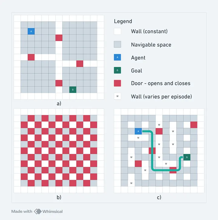
This is a fixed maze environment, which means the model can learn an optimal policy for just this one maze, and isn’t expected to navigate in other mazes. The four-rooms maze has been used in several previous RL papers (“Between MDPs and semi-MDPs: A framework for temporal abstraction in reinforcement learning” by Sutton et al, and “Hindsight Policy Gradients” by Rauber et al) as an example of a sparse-rewards problem — there is no reward shaping to hint how to solve the problem. The Agent must navigate from one random start location to a random goal location. The doorways make it improbable that the agent will randomly move between rooms, unless guided by learned preference.
We added four random doors to these doorways. Only one door is closed at a time. Which door is closed is randomly changed with probability p=0.05. This means that when a door is closed, it tends to stay closed for many time-steps, often making an different path a better option. Due to the arrangement of the rooms, there is always an alternative path to the goal when a door is closed (see figure 2):
Environment 2: Random mazes with multiple closed doors
This maze begins with a regular grid of permanent walls, with N=10 random walls and M=5 random doors (both of which can only be added at the red squares in figure 2b). The random walls are added at the start of each episode and do not change during the episode. The random doors are added at the start of each episode, but independently, randomly open and close during each environment update. The probability of a door opening or closing is 0.05.
We used A* path planning to ensure that there is at least one path which sometimes exists between the start and the goal, after the random walls have been added. However, it is possible that no path exists at times when certain doors are closed.
Learning to Plan or simply learning an optimal policy for the Environment?
The purpose of environment 2 is to force the agent to learn to plan in response to a novel maze rather than having simply learned the optimal policy for the fixed maze of environment 1. However, if you think about it, the difference between planning and an optimal policy for a superset of maze environments is … murky.
By having a very large number of possible mazes it reduces the probability that the Agent has learned the optimal path for all of them, and increases the probability that it instead learns to dynamically generate paths in response to novel mazes. Keeping the model parameter count small also makes learning a planning capability more feasible than learning all the possible mazes.
But even in the case where an Agent generates the entire route in one go (like in the original HRM maze-navigation experiments) it’s not clear that what it’s doing is planning. One definition of planning in a RL context is “use of a model of the environment in order to find a policy that hopefully will help the agent to behave optimally”. In HRM, we hope this “world-model” is being evaluated in the recurrent forward process, but we can’t observe it directly.
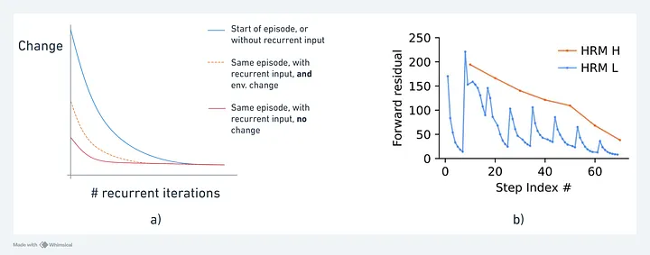
In our experiments we are using the change in the recurrent state z_H and z_L to detect changes in the model’s plans. We hypothesize that the planned route to goal is encoded in these vectors, even though the Agent only moves one square at a time. This is because in both environments the best next action depends on a distant, viable path to the goal. Therefore:
- When the environment changes in a way which makes the current plan non-viable, we predict a large change in z_H and z_L (see figure 3a, above).
- If the environment changes in a way which does not affect the current plan, we predict a small change in z_H and z_L.
- At the start of an episode, z_H and z_L are initialized to zero and we predict a large initial change from this value.
As shown in figure 3a we can plot “change” as the root-mean-squared difference between the initial value of z_H (held over from the previous timestep) and the final value of z_H after convergence. By definition, the last comparison point will have a “change” of zero.
If our predictions are correct, it will support the hypothesis that the Agent is using its internal “world-model” to produce a plan, and then generating an action for the current environment step from this plan.
The HRM-Agent model
Having discussed the environments and analysis of our Agent it’s finally time to discuss the model we have implemented. For these experiments we have used one of the simplest possible RL models, which is a Deep Q-Network (DQN) with an Epsilon-Greedy exploration strategy.
The model is trained entirely with RL; there is no supervised loss, labels or targets. Both environments provide a reward of 1 if the Agent reaches the goal, -0.01 for hitting a wall or closed door, and 0 otherwise.
The HRM model is adapted into an Agent in the simplest way we could think of: The output “head” is replaced with a two-layer dense network which is our DQN. We removed the Adaptive Computation Time (ACT) component because (as discussed above) we wish to analyse the convergence of the recurrent state z_H and z_L. This component could be restored for more efficient use of the HRM-Agent.
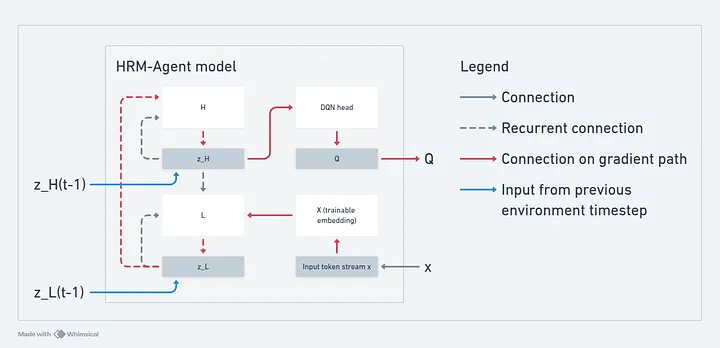
The model now has two “time-like” dimensions: Environment time, and recurrent time. The original HRM model only has “recurrent” time, because the problems are static.
The HRM model already re-uses z_H and z_L over the recurrent iterations until it halts. A single backward pass is used to update the model; there is no back-propagation over recurrent time steps.
As discussed above, it is likely that the contents of z_H and z_L from the previous environment time-step are still relevant to the current environment time-step. For this reason, we have experimented with copying these values across as the initial values used in the recurrent iterations. We have not allowed gradients to propagate into the z_H and z_L copied from previous environment time-steps.
Prior to conducting experiments it was not clear whether initializing z_H and z_L in this way would help or harm the model. We expected it would allow the HRM model to converge more quickly when any environment changes are irrelevant to its plan, efficiently reusing computation from previous environment time-steps.
But faster convergence can be limiting. We anticipated the effects on model training could be pathological, especially during the early stages of learning, when it might limit the variance of the model’s behaviour. Perhaps this issue could be ameliorated by only copying across the previous z values with probability p (similar to dropout), although so far this strategy has not been necessary.
In fact, the results we have obtained so far indicate that copying the recurrent state is actually helpful both in terms of recurrent time-to-convergence, and overall training time (measured in environment time-steps)!
Results and future work
We are now in the process of completing experiments and writing a short paper capturing this proof-of-concept of the HRM-Agent. We will also share the code.
Fortunately, we can share some preliminary results. The HRM-Agent model reaches the goal in 99%+ of episodes, in both the corridor-maze and four-rooms environments. Although these are relatively simple tasks, we believe this successfully demonstrates a PoC for training the HRM model using RL. The next question is — does the model manage to reuse its “planning” from previous time-steps, benefiting from previous computation when the environment changes?
Convergence dynamics
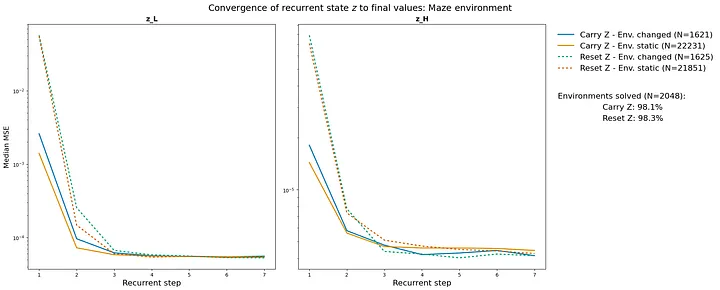
This section examines the dynamics of convergence during “recurrent time” i.e. during model “planning” iterations during a single environment time-step. We analyzed four conditions in both environments.
The four conditions were:
- Carry Z: “Re-seeding” the recurrent state (copying z_H and z_L from the previous environment time-step); environment has changed (the location of a closed door has changed, potentially invalidating the plan).
- Carry Z: “Re-seeding” the recurrent state; environment has NOT changed. The previous “plan” should be applicable to this step.
- Reset Z: Not “re-seeding” the recurrent state; environment has changed.
- Reset Z: Not “re-seeding” the recurrent state; environment has NOT changed.
In each condition, we measure the root mean square distance between the initial recurrent state (after one forward pass of the model) and final values of the recurrent state. These distances are averaged from many sample steps from many episodes (N).
The results are shown in figure 5, below:
Although these tasks and plans are very simple, this does suggest that the model can benefit from the “planning” it performed in previous environment time-steps:
- Changing the environment increases the number of iterations and distance to convergence in all conditions
- Re-seeding the recurrent state reduces the number of iterations and distance to convergence in all conditions
A greater distance to convergence implies that the initial and final “plans” are less similar. These results suggest that “re-seeding” helps improve the continuity of plans between environment time-steps, potentially improving model navigation performance overall. So, does re-seeding shorten episode length (number of steps to goal)?
Training dynamics
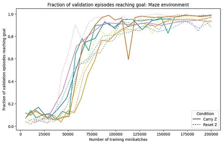
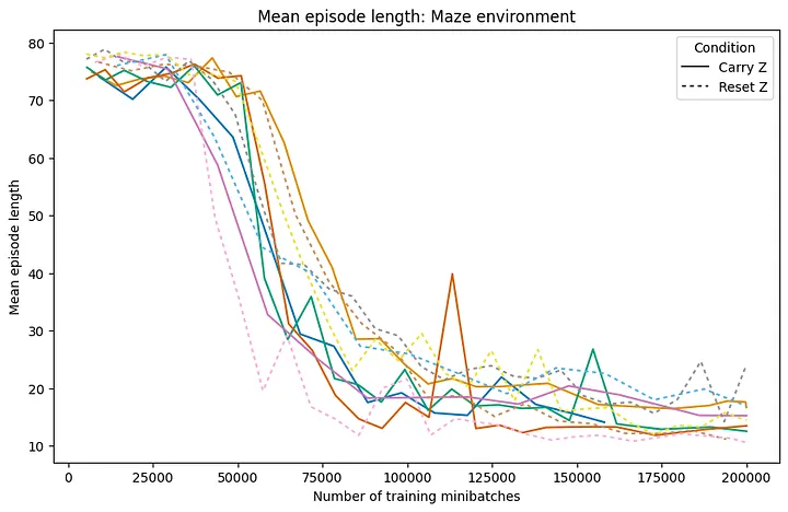
Figure 6 below shows five training runs in the maze environment with and without “re-seeding”. We don’t have enough runs yet to measure the distribution of these performance metrics so they are presented individually. In 4 of 5 training runs, re-seeding helps the model to reach 99%+ navigation success earlier in training, and also produces more efficient paths earlier in training (measured as average episode length — figure 7):
Future work
After completing the PoC paper we plan to move to partially-observable environments, allowing the agent to maintain a moving window of historic observations and reason about them. This will increase its uncertainty about the state of the environment and create a need for exploration as part of its policy.
We also intend to replace the DQN output “head” with on-policy A2C heads. This will allow more effective exploration and use of more sophisticated action spaces.
Both changes will allow the model to be used in more complex tasks and environments.
Watch this space!